Introduction to osmprob
Andreas Petutschnig
2017-07-27
Abstract
When using routing algorithms to model movement on a graph, one is not necessarily interested in obtaining the least-cost, but the most realistic results. The average path between any two points is likely never the shortest, yet there is currently no way to estimate the course or lengths of realistic paths. Instead, movement is often assumed to be singular and repeatable. osmprob is an R library that provides routing probabilities along all possible paths between any two points. The path of highest probability is the shortest, yet all edges will generally have non-zero probabilities of being traversed. Importantly, the resultant network enables calculation of the probabalistically most likely distance travelled between any two points. The package comes with a built-in Shiny Leaflet application to display the results in a matter that is both understandable and visually pleasing.Introduction
osmprob is an R package that allows users to calculate traversal probabilities and the estimated travel distance between two points on a graph based on the methods introduced in Saerens et al. (2009). It is intended to serve as a tool for researchers in fields related to city planning, logistics or transportation in general. With it, they can estimate realistic travelling distances and patterns by simply executing a few lines of code. The package also contains methods that simplify the process of downloading and preprocessing road data on which the routing can be performed. This step also includes weighting the edges according to a specified means of transport. The values used for weighting are derived from the Routino weighting profiles1, but can also be adjusted manually. Finally, the results can either be visualised with built-in mapping functions or used for further analysis.
R packages
R is a programming language that is maintained by the R Foundation for Statistical Computing2 and is freely available under the GNU General Public License. R uses the concept of packages, which allow users to access additional functionality from external sources. These packages are written and maintained by numerous contributors and can be accessed via the Comprehensive R Archive Network (CRAN)3. The packages are built according to a specific structure, which is explained in Wickham (2015), which leads to high interoperability of the contributed software. This software was also built in form of a package. One reason why this format was chosen was because of its interoperability. R is platform independent an can therefore be used on the most common operating systems. Its free software license and therefore the availability of all source code to the user, makes it an excellent research tool, as it allows all results to be completely reproducible. Looking at papers like Baker (2016), that focus on problems with the reproducibility of other scientists’ experiments, the necessity of such scientific practices becomes apparent.
Nomenclature of routing results
“path noun | \ˈpath, ˈpäth\ […] a sequence of arcs in a network that can be traced continuously without retracing any arc”
Merriam-Webster.com (2017a)
“route noun | \ˈrüt, ˈrau̇t\ […] an established or selected course of travel or action”
Merriam-Webster.com (2017b)
Usually, the results produced by routing software like implementations of Dijkstra’s algorithm as described in Dijkstra (1959) are least-cost edge sequences called paths or routes. An overview about routing algorithms can be found in Hall (2012). And whilst some of these rely on probabilities in order to simulate realistic route choice behaviour, the eventual routing results are still paths. Implementations of the Cross-Nested Logit, Probit and the Logit Kernel model can be found in Ben-Akiva, Ramming, and Bekhor (2004). It is important to clarify that the routing results produced by osmprob are not paths, but a set of traversal probabilities of all edges on the graph and other values derived from that. For lack of more fitting terminology, they will be referred to as routing results in this paper.
Road data
The road data used in this package is taken from the OpenStreetMap project, a platform that provides open geodata on a global scale. It is maintained by the OpenStreetMap contributors (2017). The data is downloaded using the osmdata package, which acts as an efficient handler for the Overpass API4 and conveniently downloads and formats OpenStreetMap data and can therefore be seamlessly integrated in the routing workflow. The package is authored and maintained by Padgham (2017).
Methods
The methods used in this paper include several steps of data preprocessing and finally the routing functionality. As this paper focuses on more the osmprob package as a whole and not on the routing methodology itself, an in-depth discussion of Saerens et al. (2009) is omitted at this point.
Preprocessing
The OpenStreetMap road data can not be used in its raw form by osmprob, but has to be preprocessed first in order to produce robust results and to minimise calculation time. According to Dasu and Johnson (2003), data preprocessing in data analysis takes up 80% of the time, which shows that it is worthwhile to invest in the development of a robust and efficient means of data preprocessing. For this reason, osmprob features a completely automated preprocessing routine, that allows users to input coordinates of a desired region and have the entire download and data cleaning process run in one go. The computationally expensive parts of this process were implemented in C++ using the Rcpp package, which brings large improvements in performance, as has been shown by Eddelbuettel and François (2011). The preprocessing process includes three steps:
- Identifying and isolating the largest connected component in the graph
- Removing vertices that are not needed to preserve the graph’s topology
- Mapping the edges of the processed graph back on to the original graph
As there was no software available that performs these steps reliably and highly performant, they had to be implemented as a part this package. The following sections illustrate the details of each preprocessing step.
Identifying largest graph component
Graph based routing algorithms do not work on a disconnected graph. But when downloading subsets of OpenStreetMap data based on a bounding box, the resulting graph may consist of several disconnected smaller graphs or components, as illustrated by the different colours for the vertices showed in figure 1. In this example, the graph consists of four components, so three of them are going to be removed in this process. One way to obtain a single connected component, is to number all separate connected components inside a bounding box individually, then pick the one component best suitable for the routing process and delete all others. In this package, the selection is based on the number of vertices in the component, which is practical for most routing applications.
Figure 1: Original data, consisting of different graph components
The following sample of pseudocode illustrates how the largest graph component is identified.
    component_number = 0

    # initially, set all component numbers to -1 (invalid)
    for vertex in all_vertices
        comp_num.at (vertex) = -1

    for vertex in all_vertices
        set component_numbers # initialise empty set of component numbers

        # insert component numbers of current and all neighbouring vertices
        component_numbers.insert (comp_num.at (vertex))
        for neighbour in vertex.get_neighbours ()
            component_numbers.insert (neighbour)

        # identify biggest component number of current neighbourhood
        largest = max (component_numbers)

        # component number is -1, so this neighbourhood is not in the list yet
        if largest == -1
            largest = component_number
            component_number++

        # assign largest component number to current vertex and its neighbours
        comp_num.at (vertex) = largest
        for neighbour in vertex.get_neighbours ()
            comp_num.at (neighbour) = largest

        # every vertex with a component number listed in component_numbers gets
        # the largest component number, thus combining previously disconnected
        # components
        for cn in comp_num
            if (component_numbers.contains (cn) && cn.component_number != -1
                comp_num.at (cn) = largest

    # remove remaining vertices
    for com in comp_num
        if com != largest
            allVertices.erase (com)
At this point every node in the graph has been assigned a component number. Nodes sharing the same component number are necessarily part of one connected unit and are disjoint from any nodes with different component numbers. Therefore, the component number with the highest frequency cmax is indicative of the largest connected component. Now all nodes with component number != cmax can be stripped off the original graph, which results in exactly one connected graph.
Figure 2: Identifying largest component
Removing intermediate nodes
All nodes that are not necessary for routing are removed from the graph. This means that nodes that only have two neighbours and are connected to both of them either by one-way streets or two-way streets can be removed and the original edges replaced with new ones connecting the remaining vertices. This constraint is illustrated in figure 3. Node B can be removed in graph 1) and 2), but not in 3). Applying it to the preprocessing routine ensures that all topological information of the original graph is preserved.
Figure 3: Intermediate nodes in one-way, two-way and mixed streets
Applying these rules to the input graph removes all unnecessary intermediate vertices, leaving only the vertices that will be part of the final compact graph.
Figure 4: Removing intermediate nodes
Inserting replaced edges
Removing vertices from a graph implies removing edges. In order to preserve the original graph’s topology, all edges are replaced with topologically equivalent direct edges between the remaining vertices. And even though this can lead to more edges leading to and from vertices, all edges keep their distinct IDs and can at any point be mapped back on the original graph. This way, the routing can be performed on the compact graph, whilst using the original graph’s edge weights for the calculations and later on its geographical features for visualisation. The following piece of pseudocode illustrates how vertices and edges to be removed are identified, replaced with new edges that have appropriate attributes and finally how these changes in the graph are tracked in a map of new and replaced edge IDs in order to be able to trace back what parts of the original graph are represented by their compact counterparts.
    # initialise unique edge ID of replacement edge
    new_edge_id = max (all_edges.get_ids ()) + 1

    # initialise map with replacement edge ID as key and a set of edge IDs as
    # value
    replacements = map (replacement_id, edge_id [])

    for vertex in all_vertices

        # if a vertex has exactly two neighbouring vertices, it can be replaced
        if (vertex.num_neighbours () == 2)

            # initialise values for replacement edge
            new_edge_weight = 0
            new_edge_start
            new_edge_end
            # initialise counter for number of edges to be replaced
            edges_replaced = 0

            for edge in all_edges
                # if current vertex is part of the current edge, replace edge
                if (edge.get_start () == vertex || edge.get_end () == vertex)

                    # depending on which of the two edges linked to the current
                    # vertex is selected, set new edge parameters and update
                    # neighbours of the neighbouring vertices
                    if (edge.get_start () == vertex)
                        new_edge_end () = edge.get_end ()
                        neighbour_1 = vertex.get_neighbour_from ()
                        neighbour_1.set_neighbour_to (edge.get_end ())
                    if (edge.get_end () == vertex)
                        new_edge_start = edge.get_start ()
                        neighbour_2 = vertex.get_neighbour_to ()
                        neighbour_2.set_neighbour_to (edge.get_start ())

                    # update new edge parameters
                    new_edge_weight += edge.get_weight ()

                    # update map of replaced edge IDs
                    edges_rep = replacements.get (new_edge_id)
                    edges_rep.insert (edge.get_id ())
                    replacements.set (new_edge_id)

                    # remove edge and increment edge counter
                    edge.remove ()
                    edges_replaced ++

                    # if both edges are found and removed, insert new one and
                    # remove current vertex
                    if (edges_replaced == 2)
                        replacement = edge (new_edge_start, new_edge_end,
                                            new_edge_weight, new_edge_id)
                        edges.insert_edge (replacement)
                        vertex.remove ()
                        new_edge_id ++ # increment new edge ID for next edge
Figure 5: Inserting edges between remaining nodes
Figure 6 shows a real world example of the principles outlined above. The original graph displayed in blue is replaced by the red compact graph that only contains the nodes necessary to maintain the original topology. The small disjoint part of the original graph has been removed, as it is not accessible from the main graph and can therefore not be used in the routing process.
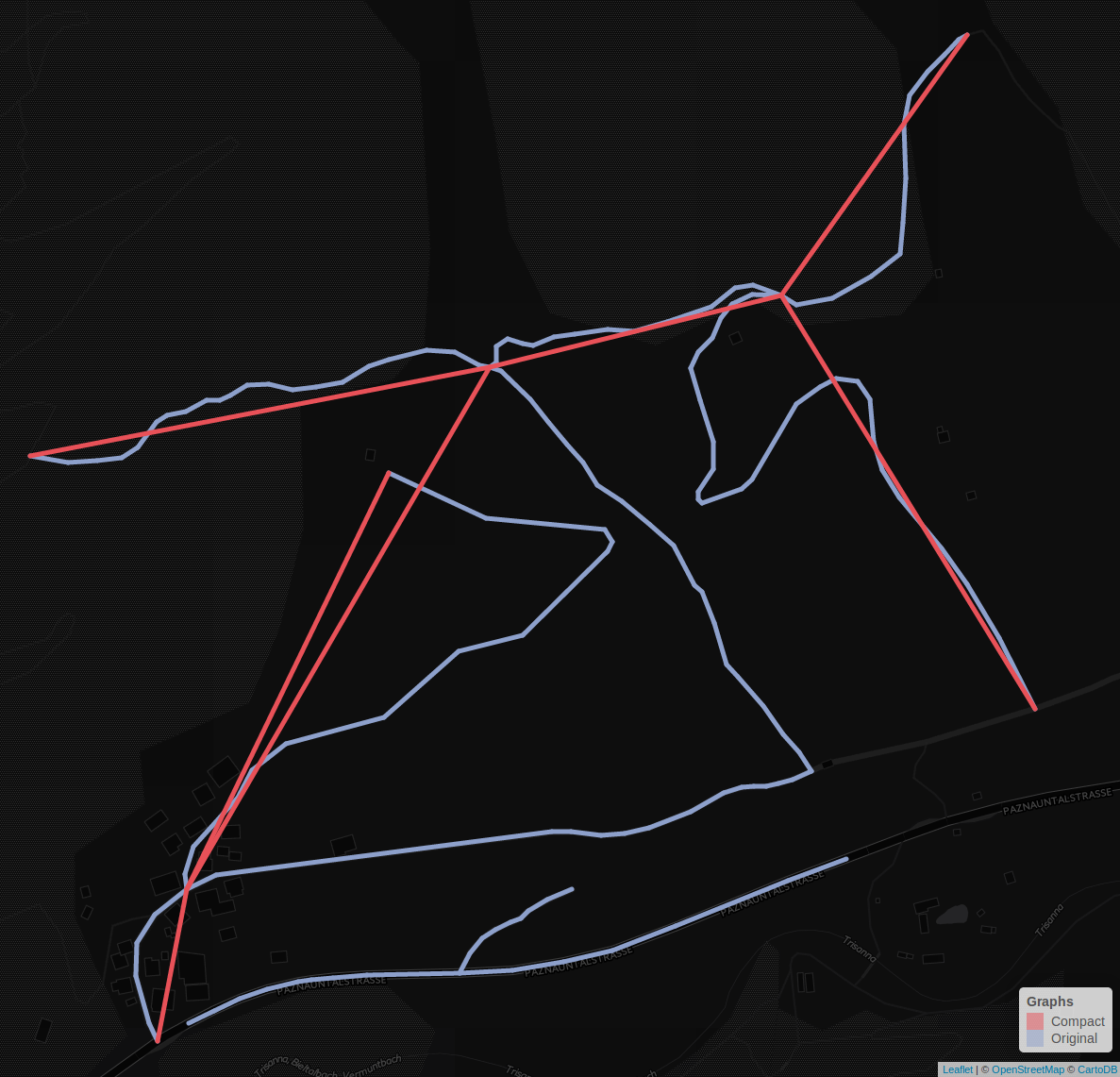
Figure 6: Comparison between compact and original graph on street data
Routing
After the preprocessing is done, the graph can be used for routing purposes. The routing function is an implementation of the methods proposed in Saerens et al. (2009). It calculates for each edge in the graph the probability of it being traversed on the way from a starting to an end point based on two factors. One is the edge weight, which in osmprob is a function of the geographic distance and the road type. The second one is a nondimensional value that Saerens et al. (2009) refer to as \(\eta\). Its value is used to quantify the global entropy that the routing algorithm uses in that for \(\eta\) approximating 0, the global entropy rises. Part of this paper is to understand the influence that different \(\eta\) have on the calculation times and routing results and how to tune \(\eta\) in a way that it leads to good routing results. Using these methods for routing leads to a probabilistic rather than deterministic routing result, which is why this routing method is fundamentally different to the ones mentioned in the introduction.
Usage
The only input needed to download street data are the coordinates of the start and end points on the graph. The download_graph function builds a bounding box including an optional buffer around the points and downloads all OpenStreetMap data tagged as key = highway5 in it.
start_pt <- c (10.5350035429,47.6034937672)
end_pt <- c (10.5384796858,47.6071612749)
graph <- download_graph (start_pt, end_pt)
The function select_vertices_by_coordinates then identifies the vertices on the graph that lie closest to the desired start and end points. These are the points based on which the routing process will be performed.
pts <- select_vertices_by_coordinates (graph, start_pt, end_pt)
route_start <- pts[1]
route_end <- pts [2]
At the moment, there are two routing algorithms implemented in this package and accessible by using get_shortest_path and get_probability, respectively. For the sake of consistency, the object returned by both functions is a list containing a data.frame with all relevant edges as a first item and the calculated distance as a second item. get_shortest_path returns the shortest path as calculated using an implementation of Dijkstra’s algorithm. The call path$d in the following example is used to access the path’s calculated distance in km.
path <- get_shortest_path (graph, route_start, route_end)
path$d # 0.1427
get_probability calculates the traversal probability for the entire input graph. It returns the entire input graph with additional columns containing the global and local traversal probability for each edge. Like get_shortest_path, it returns a list object. The first entry is a data.frame with all edge, to which have been added two additional columns. They contain the routing probabilities for all edges in two different formats:
-
prob: The local routing probabilities from every vertex to all its neighbouring vertices. These values are the ones originally calculated in the routing algorithm. The probability densities and expected mean travel distance is derived from them. Because all values ofprobadd up to 1 on a local scale, they are hard to interpret on a global scale. This is why it is also necessary to calculate the global routing probabilities. -
dens: The global routing probabilities or routing densities. These values are derived fromproband indicate how likely an edge on the graph will be traversed on the way from start to end. As these values are easier to interpret thanprob, they are used for graph visualisation.
The second item in the returned list is the expected travel distance which is based on the calculated traversal probabilities. Its minimal possible value is the length of the shortest path and gets higher with increased global entropy, which can be done using lower values for \(\eta\) (eta). Note that the distance rises very abrupt for \(\eta\) approximating 0. The results section contains more information about the effects of \(\eta\) on the routing results.
prob <- get_probability (graph, route_start, route_end, eta = 0.9)
prob$d # 0.1934
prob <- get_probability (graph, route_start, route_end, eta = 0.7)
prob$d # 0.2001
prob <- get_probability (graph, route_start, route_end, eta = 0.3)
prob$d # 0.2418
prob <- get_probability (graph, route_start, route_end, eta = 0.01)
prob$d # 1.3040
Finally, the routing results can be visualised with the shiny leaflet mapping function.
plot_map (prob, path)Results
The following section discusses the results achieved using osmprob. It also evaluates performance analysis from real world use cases and further shows the influence that different \(\eta\) have on such statistics. The tests were run on 18 different randomly selected test regions, applying 56 different values for \(\eta\) in each case. To reduce the chance of faulty outliers, the results of all speed measurements given are the median time of runs.
Routing probabilities
Figure 7 shows the probabilistic routing results on a road graph and shows very clearly the influence that different \(\eta\) have on the results. The red line on the graph indicates the shortest path between a start and end point. The line thickness on the green lines indicates the traversal probability on each edge on the way between these two points. As discussed above, high \(\eta\) mean a low global entropy and vice versa. Low global entropy means that the proposed edge traversal probabilities are higher when they are close to the ideal path. On the street network, this almost looks like the traversal probabilities resembling the shortest path. If this is the case, only very close alternative routes that don’t necessitate large detours also have elevated probabilities. On the other hand, low \(\eta\) lead to the probabilities “seeping away” from the ideal path. This can be observed by looking at the edges that are quite thin for high \(\eta\), but constantly become thicker with decreasing \(\eta\), which is consistent with the initial expectations This effect also implies that the edges with higher probabilities for large \(\eta\) will decrease in probability as the others around it will increase.
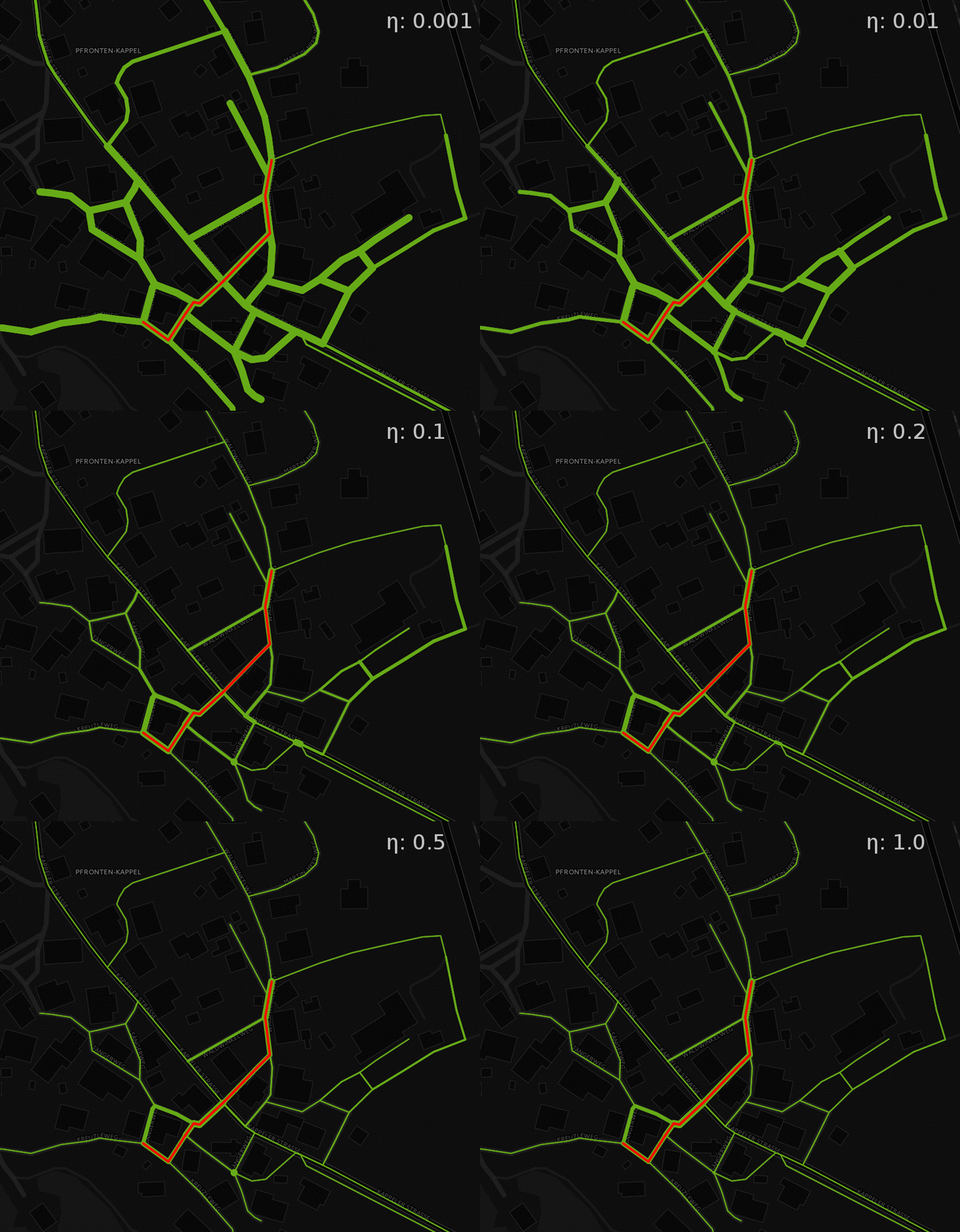
Figure 7: Varying probabilities for different global entropy parameters
Figure 8 shows the effects caused by different \(\eta\) on the routing results described above on a numeric scale. Each line represents one pair of start and end points on a graph. The coloured dots sitting on that line indicate the value of \(\eta\) used for the calculation. As stated above, high global entropy means that more edges of a graph are likely to being traversed, thereby increasing the expected mean distance of the trips. The rampant increase in expected distance also indicates that for low \(\eta\), slight changes have quite a big effect. This may even lead to estimated mean distances bigger than the sum of all edge lengths present in the graph, which is possible because random movement on the graph does not restrict the number of times a given edge can be traversed. The curves in the figure also suggest a way of extracting values for \(\eta\). The points shown in red represent the estimated ideal \(\eta\) based on the points of inflexion on the probabilistic distance data.
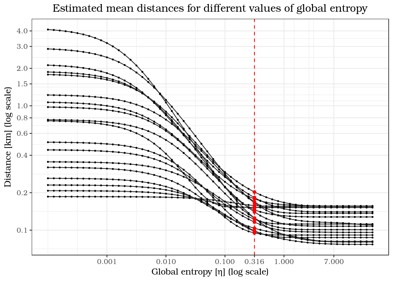
Figure 8: Mean distances for different values of global entropy
Using the estimated ideal \(\eta\) to determine the realistic mean travel distance, the median value of distances is 1.13 times the shortest distance. Because \(\eta\) is the same value for the points of inflexion in all curves, it suggests that there might be one universally applicable value for all applications. A comparison of these estimations and real world data, however would be useful to validate this.
Speed
Figures 9 and 10 show how the calculation time is affected by the graph size and the network distance between start and end point. They also give an indication of the performance difference between probabilistic routing and classic shortest path solutions at the example of Dijkstra’s algorithm. The graphs further indicate that different values for \(\eta\) may also have an influence on calculation time. Specifically, low \(\eta\) and thus high global entropies appear to be leading to longer calculation times. What becomes obvious is that the calculation times for probabilistic routing are consistently higher than the shortest path calculations, which is in accordance to the initial expectations due to the more complex nature of the probabilistic routing process. The speed tests were run using a Intel i5-2400 CPU 3.10GHz × 4 processor.
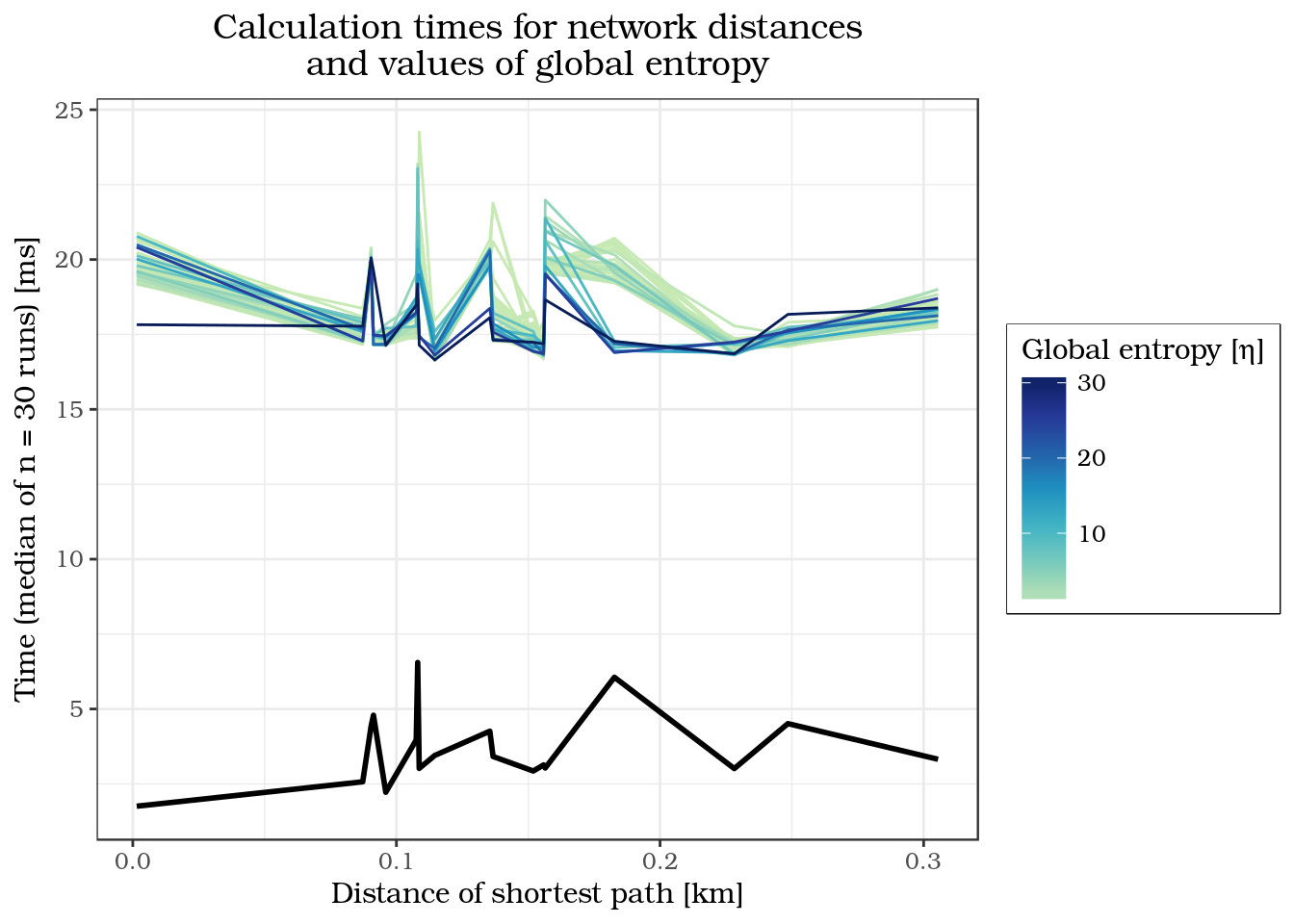
Figure 9: Calculation times for different shortest path alternatives
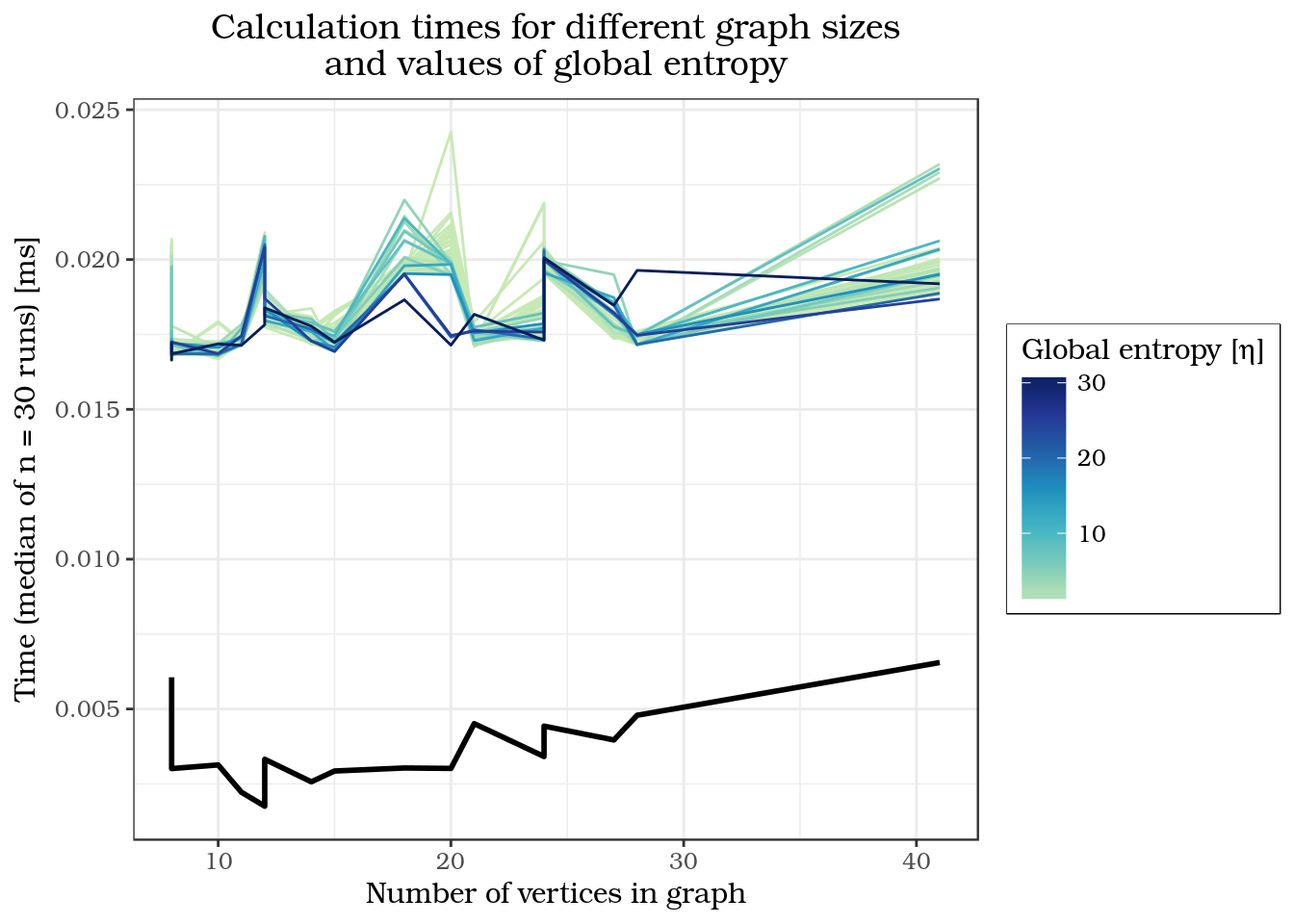
Figure 10: Calculation times for different graph sizes
Comparison with shortest path solutions
Figure 11 shows the calculated probabilistic distances for different \(\eta\) in comparison with the shortest path distances. As expected, all probabilistic distances are longer than the shortest path. The graph also shows how sensitive \(\eta\) becomes when approximating 0. Note that a change in \(\eta\) from 0.003 to 0.001 leads to an estimated distance of almost twice the length. Another observation that can be made is that the probabilistic distances alter quite a lot from one another. Table 1 shows the standard deviations of the expected distances for different \(\eta\), which are very high in comparison with the standard deviation of the shortest paths (0.068). And like the distances, their standard deviations are very sensitive to \(\eta\). Another possible reason for the spikes in the probabilistic distances could be the number of vertices in the road graph, because a more complex road graph would allow more movement between a start and end point than a very simple one would. So on a very simple graph, all movement would be restricted on few edges, even with high \(\eta\).
| eta < | Standard deviation [km] |
|---|---|
| 0.0004 | 0.0289 |
| 0.0013 | 0.0294 |
| 0.0045 | 0.0294 |
| 0.0158 | 0.0376 |
| 0.0566 | 0.0870 |
| 0.1995 | 0.2277 |
| 0.7126 | 0.5038 |
| 2.5119 | 0.8145 |
| 8.9716 | 1.0007 |
| 31.6228 | 1.0726 |
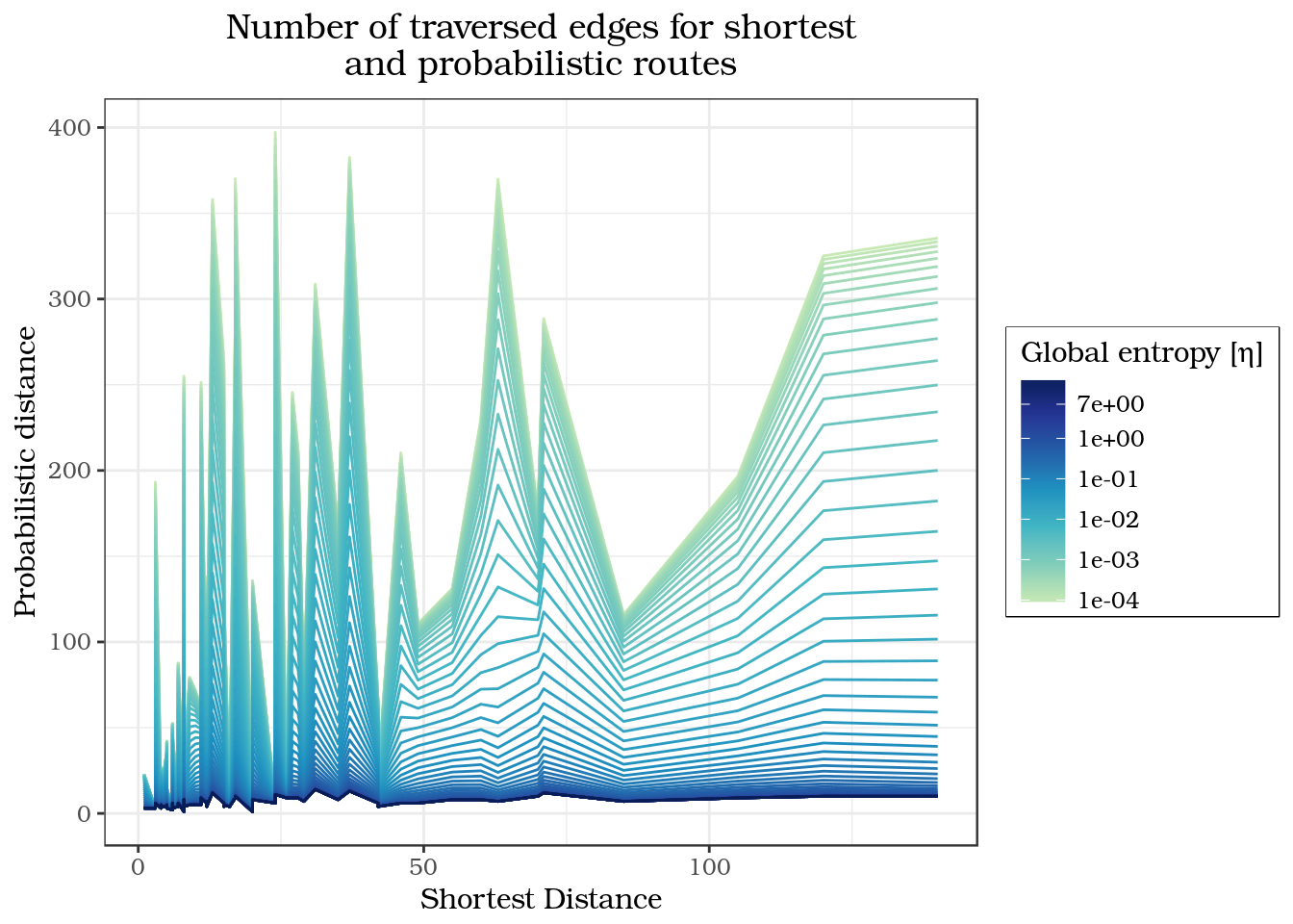
Figure 11: Comparison of probabilistic and shortest path solutions: distance
Limitations
In some test regions it was not possible to calculate probabilistic routes due to unexpected behaviour of osmprob. This includes program crashes, as well as the generation of unreasonably high values of estimated travel distances. The reasons leading these effects are yet to be identified. One possible explanation could be that under certain circumstances the software is attempting to perform routing on ill-formed graphs. This may happen when a graph is complete, but certain vertices are inaccessible due to directed edges leading only away from and not towards them. But despite these issues, the software performed as expected and could be used to produce viable results.
Discussion and outlook
The results show that osmprob can be used to not only adequately perform probabilistic routing tasks and is therefore fit for use in real world applications, it also supports the user in the process of data collection and preprocessing. This makes it very easy also for inexperienced users to facilitate the methods presented in this paper. The resulting traversal probabilities appear to represent realistic movement patterns for their respective \(\eta\). The method for estimating \(\eta\), however, is still to be investigated further. While the method of estimating \(\eta\) based on the behaviour of mean distances suggests good results, a comparison with real world movement data would be useful to validate and refine it.
References
Baker, Monya. 2016. “1,500 Scientists Lift the Lid on Reproducibility.” Nature 533 (7604): 452–54.
Ben-Akiva, Moshe E, M Scott Ramming, and Shlomo Bekhor. 2004. “Route Choice Models.” In Human Behaviour and Traffic Networks, 23–45. Springer.
Dasu, Tamraparni, and Theodore Johnson. 2003. Exploratory Data Mining and Data Cleaning. Vol. 479. John Wiley & Sons.
Dijkstra, Edsger W. 1959. “A Note on Two Problems in Connexion with Graphs.” Numerische Mathematik 1 (1). Springer: 269–71.
Eddelbuettel, Dirk, and Romain François. 2011. “Rcpp: Seamless R and C++ Integration.” Journal of Statistical Software 40 (8): 1–18. http://www.jstatsoft.org/v40/i08/.
Hall, Randolph. 2012. Handbook of Transportation Science. Vol. 23. Springer Science & Business Media.
Merriam-Webster.com. 2017a. “Path.” https://www.merriam-webster.com/dictionary/path.
———. 2017b. “Route.” https://www.merriam-webster.com/dictionary/route.
OpenStreetMap contributors. 2017. “Planet dump retrieved from https://planet.osm.org.” https://www.openstreetmap.org.
Padgham, Mark. 2017. Osmdata: Import Openstreetmap Data as Simple Features or Spatial Objects. https://cran.r-project.org/package=osmdata.
Saerens, Marco, Youssef Achbany, François Fouss, and Luh Yen. 2009. “Randomized Shortest-Path Problems: Two Related Models.” Neural Computation 21 (8). MIT Press: 2363–2404.
Wickham, Hadley. 2015. R Packages: Organize, Test, Document, and Share Your Code. “ O’Reilly Media, Inc.”